Modern video generation relies on diffusion transformers, but attention scales quadratically so pixel space calculations are intractable. A VAE (Variational Autoencoder) solves this by compressing images and videos into a compact latent space for the diffusion model to operate in. Today we're open-sourcing our Image-Video VAE, our experiment logs, and a key finding: better compression doesn't always track with VAE stability or downstream generation quality.
We spent July through November of 2024 training our own Image-Video VAE — fighting through months of NaNs, mysterious splotches, and co-training instability in the pursuit of better reconstruction quality, which (as it turns out) isn't as important as we thought.
While we ended up using Wan 2.1's VAE for our most recent text-to-video model (more on that later), we still think there's a lot to learn from the process of building a VAE given how important they are to latent diffusion models.
Today, we're releasing our Image-Video VAE and digging into the gory details: how we built it, what broke along the way, and how we're approaching our next VAE in 2026.
Linum Image-Video VAE Reconstructions


Why build a VAE?
As of today, the best generative image and video models rely on diffusion to iteratively transform random Gaussian noise into samples. These models either produce tokens one at a time or all at once in parallel. Either way, transformers are the backbone. So, we're paying the cost of attention, which scales quadratically with sequence length.
That gets expensive fast. Take a 720p, 5-second video at 24 FPS:
110M tokens for a short clip is absurd.
To make the problem tractable for the diffusion transformer, we need to compress images and videos into a smaller, continuous latent space. That's where VAEs come into play.,
A crash course on VAEs
An autoencoder compresses an input into a smaller representation through an encoder, then tries to reconstruct the original from through a decoder. The bottleneck forces the model to compress effectively and learn what actually matters about the input.
A Variational Autoencoder (VAE) adds one twist: instead of encoding each input to a single point , the encoder outputs the parameters of a probability distribution over .
VAE Inference Pipeline
In practice, we shove a data sample through the encoder to get a mean and standard deviation for each latent dimension. This defines a Multivariate Gaussian, from which we sample and push it through the decoder to get our reconstruction .
To train a VAE, we minimize the following loss:
: The KL term pushes the encoder's latent distributions towards a simple, sampleable distribution (i.e., unit normal). Typically, we set the KL weight to near-zero (1e-6). We don't care about sampling from the latent space; we just want a smooth, continuous compression. This makes our VAE essentially a very lightly regularized autoencoder.
: The reconstruction term is negative log-likelihood — in our case, an L1-style loss with a learned confidence parameter.
and : VAEs tend to produce blurry reconstructions if you only optimize KL and reconstruction losses. To fix this, we staple on two additional terms. Perceptual loss runs both the original and the reconstruction through a pretrained VGG network and minimizes the difference in their hidden representations. If two images look similar, they should have similar features even if the exact pixels don't match. Adversarial loss is borrowed from GANs to force details into the reconstructions. We train a discriminator to tell real images from reconstructions, and the VAE tries to fool it.
When training text-to-video models, you first need to pretrain the model on image generation. The model needs to understand nouns (people, places, things) before it can understand verbs (actions, motions, camera movements). Since our VAE needs to handle both images and videos, our loss function becomes the sum of image and video losses:
Building a baseline – a working video VAE [1 week]
In Fall 2024, there were no good open-source Video VAEs (let alone Image-Video ones), so we started with the simpler problem – video only. We used a traditional CNN Encoder/Decoder style architecture, swapping Conv2Ds with Conv3Ds.
Linum VAE Architecture
FLUX-1 used 8x spatial downsampling (i.e., 3 × 256 × 256 image to C × 32 × 32 latent), but we didn't know what would be optimal for video. So, we started off conservatively and used a 4x spatial downsample and 4x temporal downsample.
4x Spatial, 4x Temporal Compression (324p, 1 second)
Reconstructions are visually identical to the originals — no obvious artifacts at 4x compression.
It worked out of the box (encouraging, given we'd never trained a VAE before), but it was way too little compression to be useful. At 4x compression, we were unable to fit a single 360p, 1-second video clip in memory without OOM-ing on an 80 GB H100.
We traced super-linear memory growth to the AttentionBlock in the Encoder and Decoder. There were two obvious fixes: downsample more before hitting the AttentionBlock or train with FSDP. Since 8x spatial downsampling clearly worked in FLUX-1, we opted to push compression harder and ran a few experiments:
| Spatial Downsample (H, W) | Temporal Downsample (T) | Effective Compression | Result |
|---|---|---|---|
| 4x | 4x | 12x | Unusable — insufficient compression at higher resolutions |
| 8x | 8x | 96x | Unusable — bad reconstructions |
| 16x | 4x | 192x | Unusable — bad reconstructions |
| 8x | 4x | 48x | Usable — rare artifacts at 180p, typically high-motion |
Effective Compression Rate = Height Downsample × Width Downsample × Time Downsample × (3 RGB channels / 16 latent channels)
Right now, latent size is mechanically tied to input resolution, not content complexity. Ideally, our compression would take into account the complexity of the video itself when determining the embedding size. For example, a video of a placid lake contains less information than a video of a boxing match. It doesn't make sense that they have the same latent size, even if the videos have the same size and duration.
Co-training on image and video [3 months]
Getting a working baseline typically takes a lot longer, so we were pretty stoked to see so much progress in just one week. And then (as always), we hit a wall …
Handling 1-frame (image) and k-frames (video)
To handle single-frame images, we padded each image into a 4-frame "static video", which the temporal downsampling reduced back to a single latent frame by the bottleneck. Out of the gate, the video reconstructions looked fine but the image reconstructions were unusable.
Naive Co-training: Blurry Image Reconstructions
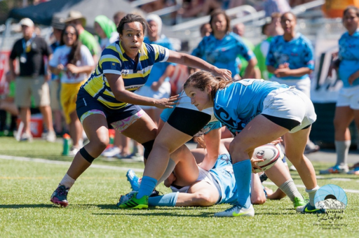

Rugby player's face is missing a lot of detail. Features are smeared and indistinct.


Our first hunch was that our "static video" approach to image reconstruction might be unstable, so we re-trained the network on just images. That worked just as well as the video-only VAE, so we started digging into the loss function to debug why co-training was leading to worse reconstructions.
Death by summation – accidentally washing out our image signal
Our reconstruction loss summed over all dimensions () then divided by our batch size ():
With this formulation, loss magnitude scales linearly with tensor size. That's a huge problem, because images and videos have very different sizes.
A 180p, 2-second video at 24 FPS is . A 256×256 image (repeated 4 times for our static video trick) is . The video contributes ~10x more to the loss — not because it matters more, just because it's bigger. As a result, we're essentially making the optimizer blind to images altogether.
The naive fix (mean per sample) normalizes this away:
But now, the gradient per pixel is inversely proportional to tensor size. A single bad pixel in the 256×256 image drives ~10x more gradient than the same bad pixel in the 180p video. This places way too much emphasis on picture-perfect image reconstruction.
To combat this problem, we kept the original sum-based loss but normalized it relative to a fixed reference shape, :
This kept loss magnitude consistent across resolutions without distorting per-pixel gradients and allowed us to explicitly re-weight the importance of different resolutions and modalities.
Naturally, we tried equal weight for images and videos, but that NaN-ed pretty quickly. When we backed off to lower image weights like 0.25, we were still NaN-ing ...
Co-training instability (AKA NaN Hell)
When your network is unstable, the first thing you do is look at the magnitudes (L2-Norms) of the activations and gradients. Our VAEs were obviously exploding, so we added Group Norms everywhere. This stabilized early training, but we still hit exploding gradients deep into training.
Our first thought was that the model was struggling to distinguish between the "static videos" and real ones, so we should provide an explicit signal that it was dealing with two different modalities.
To tackle this issue, we introduced FiLM (Feature-wise Linear Modulation) layers throughout the autoencoder. We took the hidden representations from the CNNs () and modulated them with a shift () and scale (), conditioned on an image/video identity embedding ():
Scale parameters would hover around 0 for the early training stages, and as soon as they became non-zero (i.e. started driving signal from the image vs. video differentiation), we would run into exploding gradients and NaN. The FiLM layers didn't help, so we axed them from the network.
Since this more "principled" architecture fix didn't work, we ran towards training stabilization "hacks", introducing our own variant of adaptive gradient clipping (AGC) from Brock et al. (2021). Rather than clipping to a fixed threshold, AGC tracks the ratio of gradient norm to weight norm per parameter using an exponential moving average and clips any channel whose ratio exceeds the learned threshold. This stabilized training, but we started seeing discolored splotches in our reconstructions.
Discolored Splotches in Reconstructions (180p)
Green splotch in bottom left and at the base of the tree on the right.
Out, damned spot!
The authors of LiteVAE (Sadat et al. 2024) ran into a similar problem, with black spots appearing in their image reconstructions. Their solution was to swap Group Norm + CNN blocks with a Self-Modulating Convolution (SMC) operation.
Instead of normalizing output activations, SMC normalizes the convolution weights. Each weight is scaled by a learned per-input-channel parameter that controls how much each input channel contributes to the output. Then the scaled weights are divided by their L2 norm, so that the CNN doesn't blow up the output activations.
Empirically, Group Norms force pixel-space-decoding-models to over-emphasize certain pieces of information through a small number of pixels. If there is a particular channel within a group that has outsized magnitude, Group Norm over-emphasizes this channel while nuking the signal in all the other channels within the group.
SMC is fundamentally more expressive. It allows the network to modulate each channel independently, while preventing activation growth. This allows the model to have more flexibility in how it propagates the higher magnitude signals, helping us avoid the spots.
By adapting SMC for Conv3Ds, we were able to get rid of the splotches in our 180p video reconstructions, but the black dots re-appeared when we started scaling to 360p and 720p videos. To pinpoint the origin of these new spots, we instrumented hooks in the forward pass of our VAE, plotted the L2 norms of each pixel-activation at each layer, and manually reviewed all the plots to find the layer where the spots first showed up.
The culprit was the AttentionBlock in the Encoder's Mid Block. We tried dropping Group Norms from the Encoder and Decoder Mid Blocks, but that was wildly unstable, so we replaced them with a lighter form of normalization, Pixel Norms.
Right after we solved this problem for ourselves, Meta published their MovieGen paper. In it, they describe the exact same problem, but they overcame it by slapping another term onto their VAE loss that penalized outlier values in their network's activations. Truth be told, we have no clue how well Meta's solution works, since they never released their models. But broadly speaking, there are definitely other solutions to this spot problem.
Training across resolutions [2 weeks]
3 months in, we had a working VAE, but the final 720p checkpoint catastrophically forgot how to reconstruct lower resolution images and videos. We need the VAE to work reasonably well across all resolutions, since we train the diffusion model across resolutions. So, our fix was to change the VAE's curriculum.
Instead of moving sequentially from 180p → 360p → 720p, we kept training on lower resolutions while introducing higher resolutions. Then, we ran a hyperparameter sweep to identify the optimal loss weights for the different resolutions, landing on a final cocktail of 180p at ~1.1 loss-weight, 360p at 0.1, and 720p at 0.01.
If it works, why switch to the Wan 2.1 VAE?
When training diffusion models, you embed your dataset once with your VAE offline. This way you don't have to incur the embedding cost every time you run a diffusion model experiment.
When Wan 2.1's VAE dropped in February 2025, we had only embedded a subset of our dataset, so we held a bakeoff. It performed just as well as ours, but it was smaller and faster since it doesn't compute full spatio-temporal attention. So, we decided to ditch our own VAE and save $ on embedding our large dataset.
Better reconstruction ≠ better generation
When we built our VAE, we obsessed over pixel-perfect reconstructions. We spent weeks sweating over the ~10% of samples our model struggled with.
Looking back, we should have just filtered out these samples from the dataset and moved on. We know that sounds counterintuitive.
Shouldn't you be robust to edge cases? Yes – but not when the edge cases are low-quality samples:
Examples of low quality image data
Heavily pixelated face. Can't clearly distinguish nose from eyes from mouth.


The most difficult images tend to be heavily pixelated. Faces are blocky and smeared; trees and foliage look like flat blobs of green, devoid of any details in the branches and leaves; and on and on. These artifacts are telltale signs of aggressive JPEG compression.
Compression artifacts are harder to reconstruct than real detail — because they're just noise. When you push the VAE to perfectly reconstruct them anyway, you contort your latent space to capture this detail. In other words, overanchor to reconstruction quality, and you're just training your VAE to regurgitate noise..
This is why co-training across resolutions was so unstable for us. The model had baked its understanding of noise into its representations at 180p and then had to completely re-shape its latent space when we introduced higher resolution data.
This poses a subtler issue for downstream diffusion models.
Intuitively, you'd think that if a diffusion model sees the world through the VAE's latent space, a sharper lens should allow it to pick up patterns more easily and generate crisper samples. Turns out, that's not the case.
In the 18 months since we trained our VAE, researchers have consistently found that VAEs with higher quality reconstructions may produce worse diffusion models. For example, Yao et al. (2025) improved the rFID of their VAE on ImageNet from 0.49 to 0.18 but the downstream diffusion model's gFID tanked from 20.3 to 45.8.
By blindly optimizing reconstruction loss in your VAE, you're overfitting to noise (compression or otherwise) and hurting the model's chance to disentangle your data into a semantically, meaningful space. You're "compressing" your data to make the attention calculation tractable, but in doing so you're making it harder for the diffusion model to learn visual concepts.
So, how do we create a "learnable" latent space? Right now, there seem to be two answers –
- Regularize the VAE, so it learns a more semantically meaningful latent space.
- Skip the VAE altogether and just train the diffusion model in pixel-space.
Option #1 is in vogue right now. The original idea comes from REPA (Yu et al. 2024), where the authors found that they could accelerate diffusion model training by aligning the generative model's hidden states to those of a pre-trained vision encoder like DINO. Since then, there has been follow-up work by Leng et al. (2025), which demonstrates that you can induce a more learnable latent space within the VAE by un-freezing the encoder and backpropagating the diffusion model's alignment loss into it. End-to-end training with a VAE is impractical for text-to-image and text-to-video models, but we could achieve similar results by re-training the VAE itself with an alignment loss in the mix (e.g. VA-VAE) or scaling up the VAE to directly learn these self-supervised representations, like in VTP. With this "alignment regularization" in place, we should be able to push better reconstructions without sacrificing learnability altogether.
Option #2 is hot off the presses and might be a peek into the future. In JIT, the authors show that we can get a diffusion model to learn the compression itself without a VAE whatsoever with a few small tweaks to the typical flow-matching learning objective (more on this in another post). The downstream generations are still worse than the best aligned-VAE samples … but give it a few months of follow-up work. Our in-house hunch is that JIT is overfitting to noise, though not nearly as much as our VAE. Perhaps, by having JIT explicitly learn semantic representations like those in DINO it'll be able to leapfrog existing approaches and make it easier for all of us to train diffusion models.
Who are we?
We're two brothers training text-to-video models from scratch. We're trying to make animation accessible so that anyone can make their own shows and movies.
We posted this over on Hacker News. Check the link, if you want to join the discussion.
Get Field Notes
Technical deep dives on building generative video models from the ground up, plus updates on new releases from Linum.